

In this blog, I am going to describe basic but useful Google Sheets formulas that you need to know. Formulas for Google Sheets are special keywords that enable you to make calculations based on the data in your Google Docs spreadsheet.
Formulas for Google Sheets can be used to perform many operations and tasks automatically. To type any formula in Google Sheets, you have to start by typing the “equals” symbol(=) followed by the name of the formula you want to use. Ready to learn how to use formulas in Google Sheets? Let’s go!
Need help in removing duplicates on your Google Sheets? Learn how here.
Basic Google Sheets formulas list:
- SPLIT
- JOIN
- FILTER
- COUNTA
- SPARKLINE
- DETECTLANGUAGE
- GOOGLETRANSLATE
- IMPORTRANGE
- CHAR(8226)
Prefer to watch a video than read? We've got you covered.
(1) SPLIT to divide text
The SPLIT formula divides the text around a specified character or string.

To use the SPLIT Google Sheet formula follow these steps:
- Click on the cell where you want to add the formula
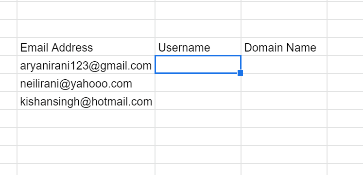
Here we are going to split the username and domain name from the email address.
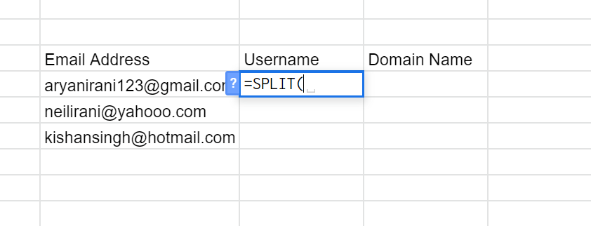
- Type =SPLIT( to start the formula
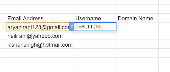
- Next, you have to specify the cell that you want to split.
- Now you have to specify the character or characters to split the cell that you have specified.

- Here we are going to split the text based on ‘@’ and get the username and domain name.
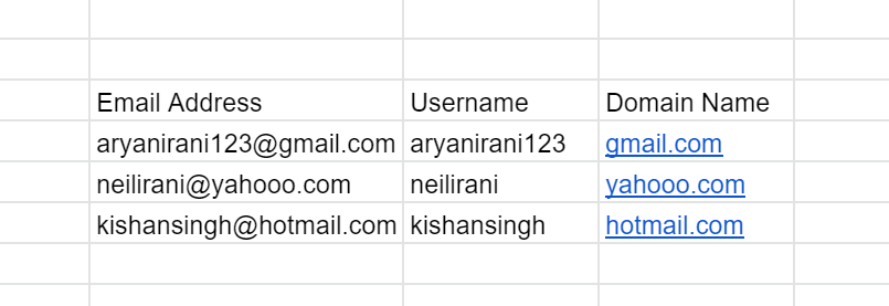
- After selecting the range and specifying the splitter , close the bracket and hit enter.
- On successful execution, you will see the following output.
(2) JOIN to combine text
The JOIN formula combines strings (data in cells), with a specified separation between the two strings.

To use the JOIN formula follow these steps:
- Click on the cell where you want to add the formula

- Type =JOIN( to start the formula

- In the JOIN formula, you have to specify the separator between the two variables that you want to join.
- To do that you have to select the first value that you want to join followed by the separator and then the second value.
- In this case, we are just going to separate the two values with space. Each value is separated by a comma (,).

- After selecting the cells you want to join, close the brackets and hit enter.
- On successful execution, you will see the following output.
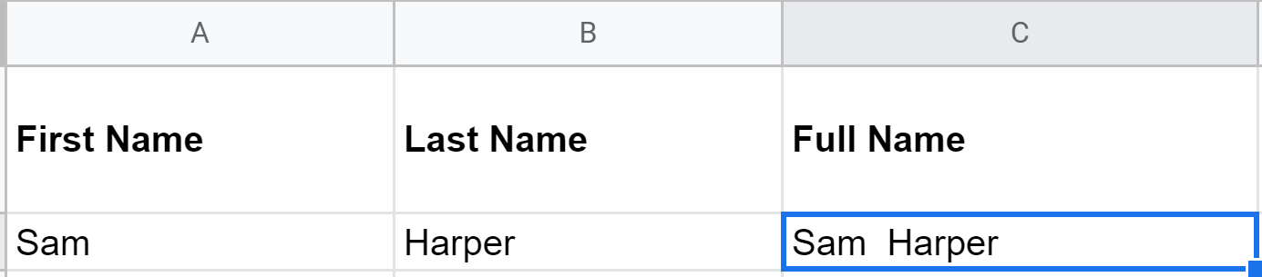
The same can be done for all the rows of data that you have.
(3) FILTER to extract data
The FILTER formula helps you extract data that meets the specified criteria.

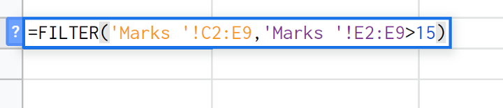
To filter the data you have to specify the range you want to filter, followed by the filter condition.
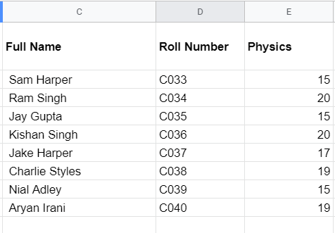
This is the data that we are going to filter. We only want the list of students who have scored more than 15 in physics.
To use the FILTER() formula follow these steps:
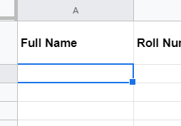
- Click on the cell you want to get the filtered data.
- Type =FILTER( to start the formula.
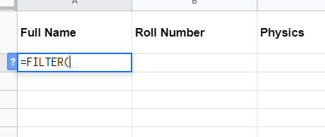
- To filter the data we have to specify the range you want to filter followed by the filter condition.
- After filling out the details, close the bracket and hit enter.
- On successful execution, you will see the following output.
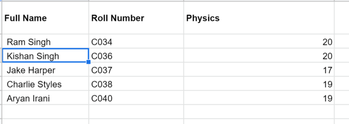
Here you can see we have only got the students names whose marks are more than 15.
(4) COUNTA for counting
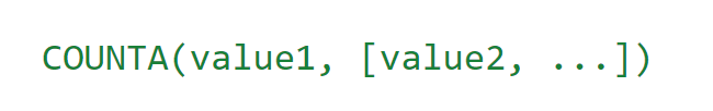
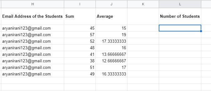
The COUNTA formula gets the number of values in the specified range. In this example, we are going to get the number of students using the CountA formula.
To use the COUNTA formula follow these steps:
- Click on the cell you want to add the formula
- Type =COUNTA( to start the formula
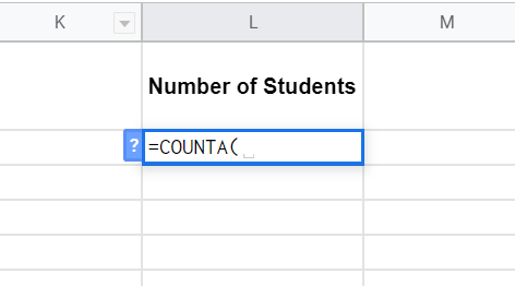
- To get the count of a column you have to specify the range.
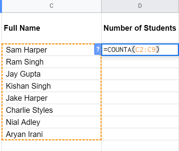
- Here we have specified the column till the end so that the count will keep increasing as soon as new names come in.
- We have started from the second row so that the header does not get counted.
- After specifying the column you want to count, close the brackets and hit enter.
- On successful execution, you will see the following output.

(5) SPARKLINE to get an in-cell chart
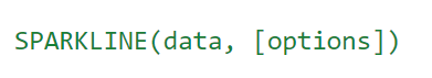
The SPARKLINE formula creates a miniature chart inside a cell for a specified range.
To use the SPARKLINE formula follow these steps:
- Click on the cell you want to add the formula
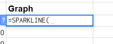
- Type =SPARKLINE( to start the formula
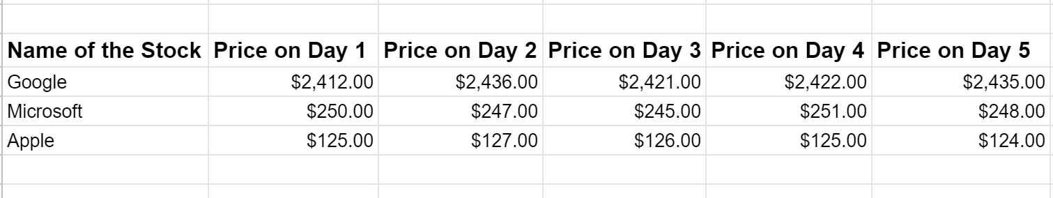
- To create the chart for each stock you have to specify the range.

- Here we have specified the range to create the chart. Suppose you want a special type of charts, such as bar, column, and more, to know more click on the link below.
- After specifying the range, close the brackets and hit enter.
- On successful execution, you will see the following output

- Here you can see that the chart has successfully been created.
(6) DETECTLANGUAGE to identify the language
The detect language formula identifies the language used in the specified range.

To use the Detect Language formula follow these steps:
- Click on the cell you want to add the formula

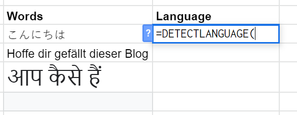
- Type =DETECTLANGUAGE( to start the formula.
- To translate the English cell, you can either enter the cell range or select it.
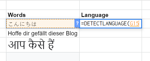
- After specifying the cell or range, close the bracket and hit enter.
- On successful execution, you will see the following output.
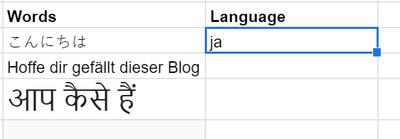
- Here you can see that the first cell is Japanese, and we have successfully detected the language.
(7) GOOGLETRANSLATE to convert text
The Google Translate formula converts text from one language to another.

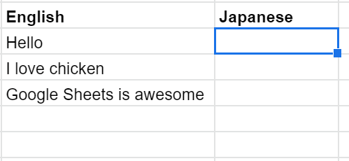
We have to first specify the text that we want to translate, followed by the current language and the target language. In this case, we have some cells in English that we want to translate to Japanese.
To use the Google Translate formula follow these steps:
- Click on the cell you want to add the formula
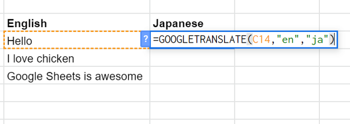
- Type =GOOGLETRANSLATE( to start the formula.

- To translate the English cell, you can either enter the cell range or select it.
- After selecting the range, you have to specify the source language followed by the target language.
- To specify the languages we have to use some specific keywords. For English, the keyword is ‘en’ and for Japanese, the keyword is ‘ja’.
- After specifying the range, source language, and target language, close the brackets and hit enter.
- On successful execution, you will see the following output.

- To know more about Google Translate keywords, check out the link below.
(8) IMPORTRANGE to get import data from another spreadsheet
The import range formula gets a range of data from a specific Google sheet.

To transfer data from one Google Docs spreadsheet to another, normally people just copy/paste but changes on the original spreadsheet won’t be replicated on your copy. Using the import range formula you can transfer data from one Google sheet to another easily while keeping your data in sync.
First, you have to put the target sheet URL followed by the sheet name and the range you want to import.
To use the IMPORTRANGE formula follow these steps:
- Go to the new sheet and select the cell where you want to import the data

- Type =IMPORTRANGE( to start the formula.
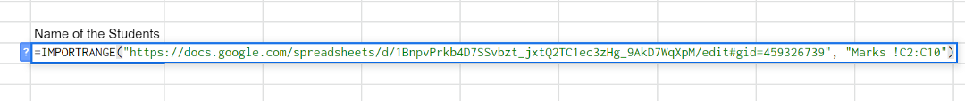
- After starting the formula you have to put in the link of the target spreadsheet, followed by the name of the sheet from which you want the data and the range of data that you want to import.
- After filling out the link, name of the Spreadsheet, and the range, close the bracket and hit enter.
- On successful execution, you will see the following output..

- Here you can see all the names have come into the Google Spreadsheet.
(9) CHAR(8226) to insert bullet points
The CHAR(8226) formula in Google Sheets creates a bullet point inside a cell followed by the specified text.
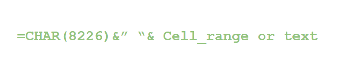
To add a bullet point you have to write the char(8226) followed by the separator between the bullet point and the text.
To use the char() formula follow these steps:
- Click on the cell you want to add the bullet point to.
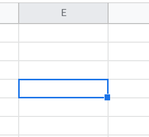
- Type =char(8226 to start the formula.
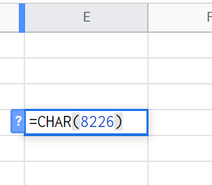
- To add some text after the bullet point, you have to specify the separator followed by the text/range.

- All the parameters are separated by &, first the char keyword followed by the separator and the text/ range.
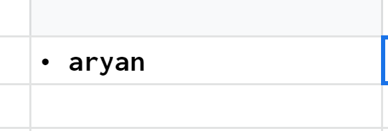
- After filling out the filling-in parameters, close the bracket and hit enter.
- On successful execution, you will see the following output.
Useful Google Sheets formulas: A summary
We have provided you with 9 basic Google Sheets formulas that will help you to make calculations based on your Google Docs spreadsheet data. I hope you now know how to use Google Sheets formulas. If you feel I have not mentioned some formula let me know what I should write next.