5 ways of checking for duplicates in Google Sheets

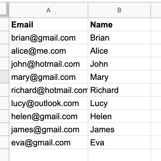
We all have wondered at some point, is there a way to find duplicates in Google Sheets? In this post, I will show you how to quickly find and delete duplicates from a Google Sheets column. If you are preparing a YAMM mail merge, it’s best to check for duplicate email addresses beforehand to avoid sending multiple emails to the same recipient. Fortunately, Google Sheets provide several easy ways to clean your list from duplicates.

How to Find Duplicates and Delete Them in Google Sheets: 5 Methods

1. Remove Duplicates feature
2. Conditional formatting
3. COUNTIF formula
4. UNIQUE formula

1.How to remove duplicates in Google Sheets

If you want to know how to emove duplicates in Google Sheets and don’t need to review duplicate values, Google Sheets have a very quick and easy way to delete any repeated values in a column.

1. Click on the Data menu and select Remove Duplicates

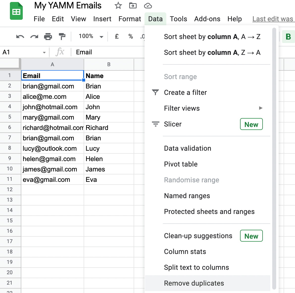
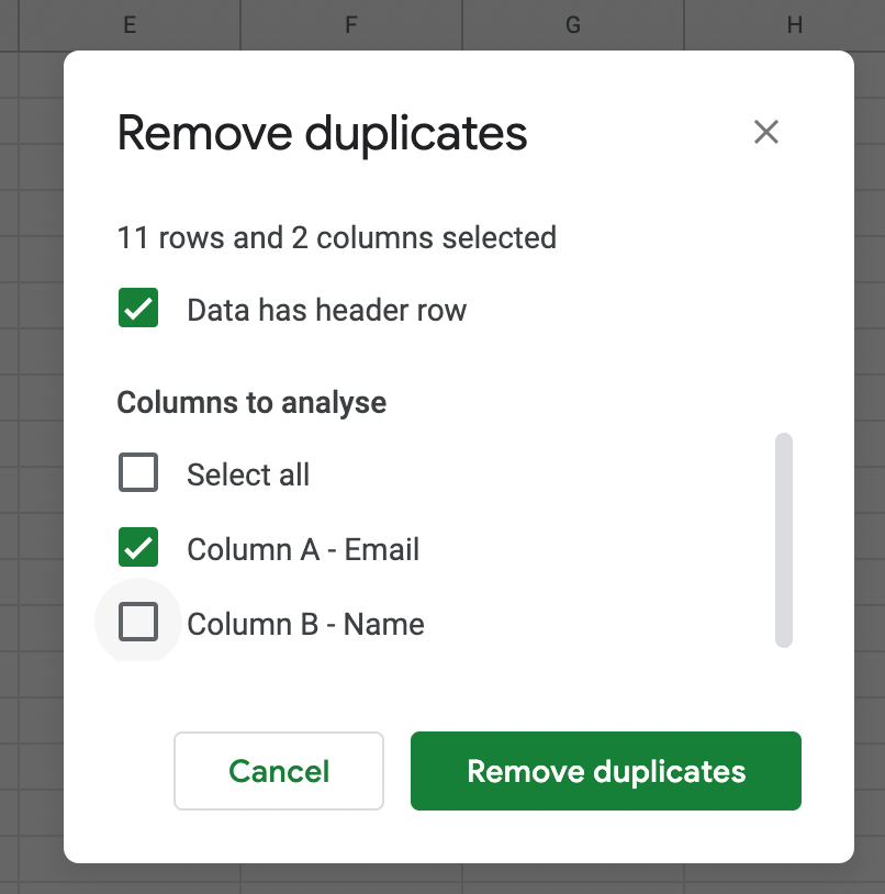
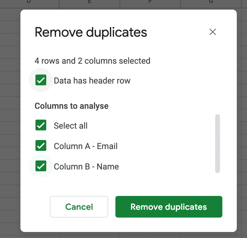
2. In the pop-up, check the box “Data has header row” (this prevents your header row from being taken into account for duplicates removal)

3. Tick the column from which you want the duplicates to be removed: in my case, it’s Column A - Email.

4. Click the Remove Duplicates button. Google Sheets will keep only the first instance of the email address and completely delete the cells with duplicates.

In the end, you will get a pop-up informing you of how many duplicates were removed and the number of rows that remain.

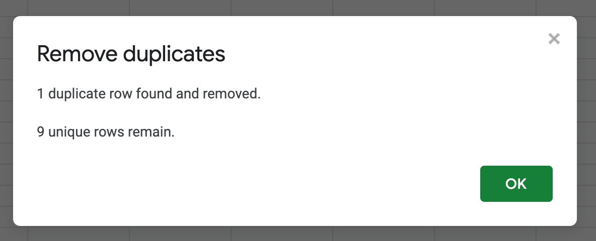
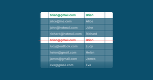
As you can see from the results, the second instance of brian@gmail.com was removed:

If you need to remove the table rows which contain the same values in all columns, make sure to check all applicable columns in the pop-up. For example, let’s say my list contains 3 rows with the same email address brian@gmail.com and two different names - Brian A and Brian B.

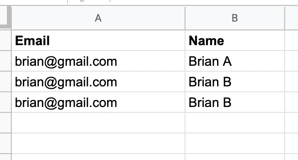
I can remove the second occurrence of the combination brian@gmail.com and Brian B by checking both Column A and Column B for duplicates removal.

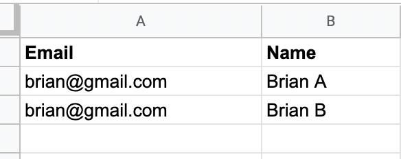
And this is the result - only one instance of Brian B is kept in the list:

2.How to highlight duplicates in Google Sheets using conditional formatting

Wondering how to highlight duplicates? Using this method, you can highlight duplicates in Google Sheets to review them. This method is just slightly more complex than the previous one.

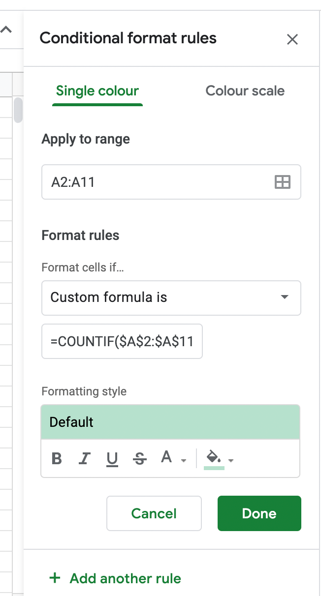
1. Select the range of cells you want to analyze and click Format -> Conditional Formatting.

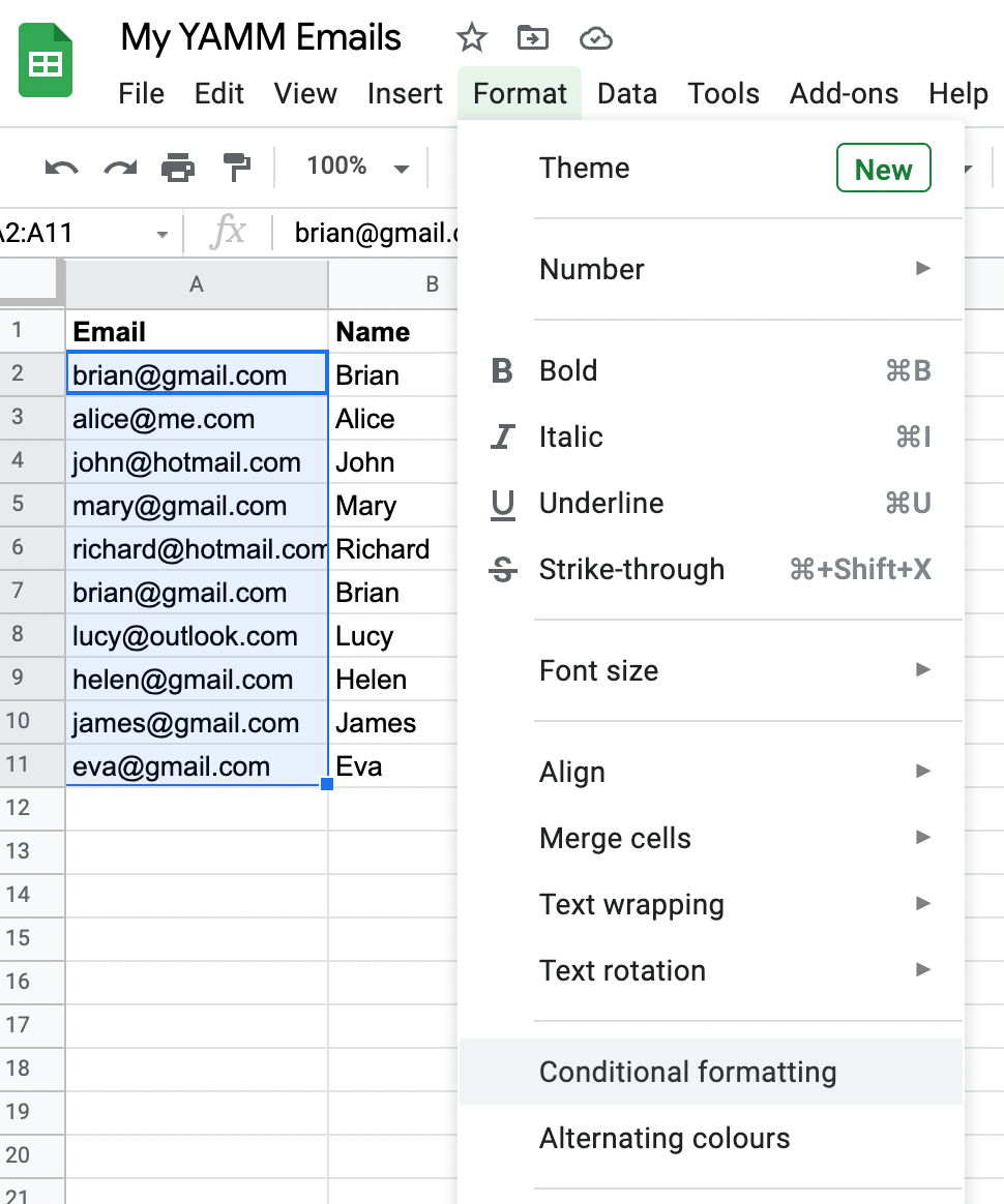
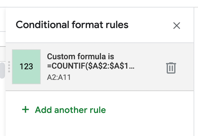
2. In the sidebar pane under the Format Rules dropdown select “Custom formula is”.

3. Introduce the following formula in the field below:

=COUNTIF($A$2:$A$11,$A2)>1

Note: $A$2:$A$11 in the formula means that Google Sheet will analyze rows 2 through 11 in Column A, and the second argument $A2 indicates that it will start reviewing from the second row. If your sheet has a different structure, you will have to change the formula respectively to highlight duplicates in sheets.

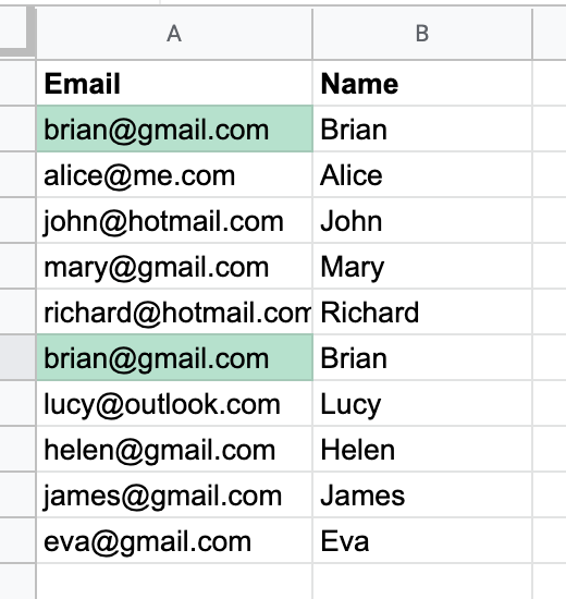
4. Click Done and the duplicate values in your list will be highlighted automatically:

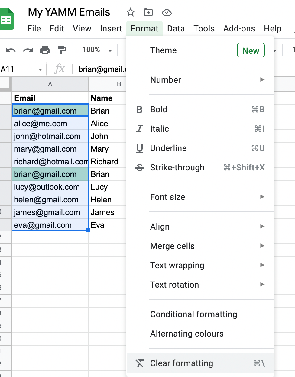
To remove highlighting:

1. Select the range of cells
2. Click Format -> Clear Formatting

You can have multiple Google Sheets conditional formatting rules for duplicates at the same time If you do have several conditional formatting rules active and want to remove one or more, you can do this in the Conditional formatting sidebar panel:

3.Deploying COUNTIF to count repeated values

This method is similar to the above, but instead of highlighting a duplicate value, you will have a separate column showing how many times a particular email address appears in a column. It is convenient in Google Sheets to filter duplicates by denoting unique and repeated values too.

1. Start by creating a new column - for example, “Number of occurrences”.
2. Introduce the following formula in the second row and drag it down:

=COUNTIF($A$2:$A$11,$A2)

Google Sheet will calculate how many times each value appears in the column: here, we can see that brian@gmail.com is repeated twice.

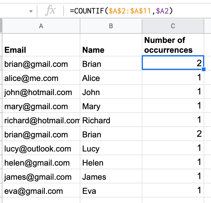
Now you can filter the sheet by values greater than 1 and analyze duplicate addresses in detail. Note that both the first and the second instances of the email address will show “2”.

Same as before, $A$2:$A$11 in the formula means that Google Sheet will analyze rows 2 through 11 in Column A, and the second argument $A2 indicates that it will start reviewing from the second row. If your sheet has a different structure, you will have to change the formula respectively.

4.How to dedupe in Google Sheets by finding the first and repeated instances

If you want to remove duplicates in Google Sheets by finding the first and repeated instances of an email address, the COUNTIF formula will save the day again.

1. Create a new column.
2. Introduce the following formula in the second row and drag it down:

=(COUNTIF($A$2:$A2,$A2)=1)+0

The first occurrence of the value will be indicated by “1”, while any repetition will appear as “0”.

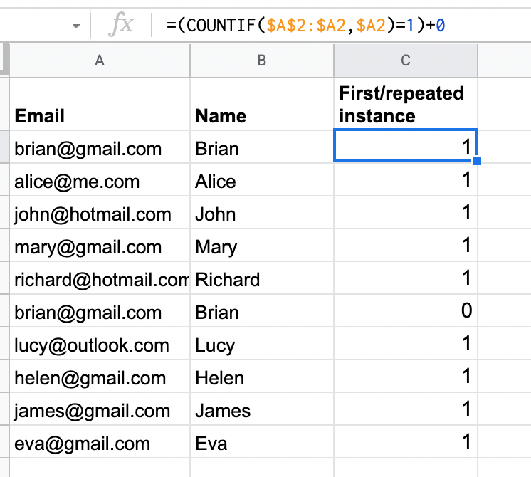
This method allows you to easily filter the sheet by the first or repeated instance. For example, you can filter in the first occurrences of the email addresses and use YAMM segmentation to send your campaign to the filtered rows only without removing any rows from your sheet.

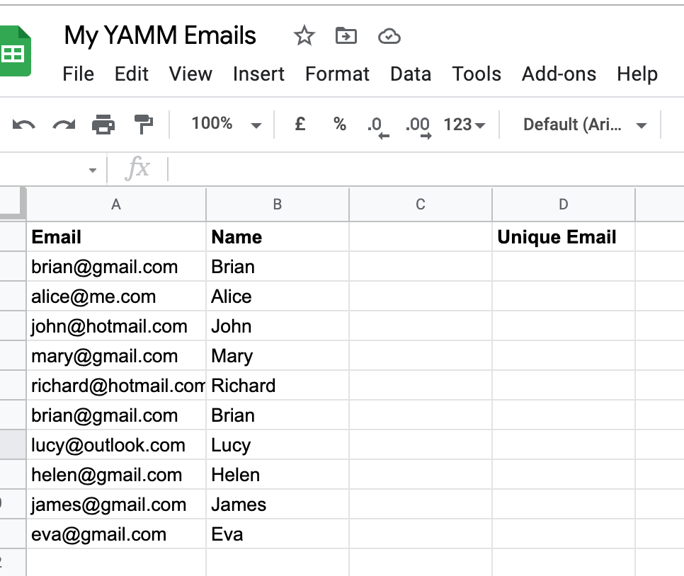
5.How to search for duplicates in Google Sheets by listing unique values in a different column

This is a simple method if rather than deleting duplicates in place, you want to pull unique values into another column or even sheet.

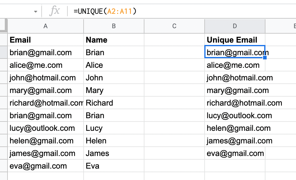
1. Start by creating a new column - I will call it Unique Email:

2. In the second row of your new column, introduce the formula:

=UNIQUE(A2:A11)

3. Press Enter. Now you have a new column with unique values only:

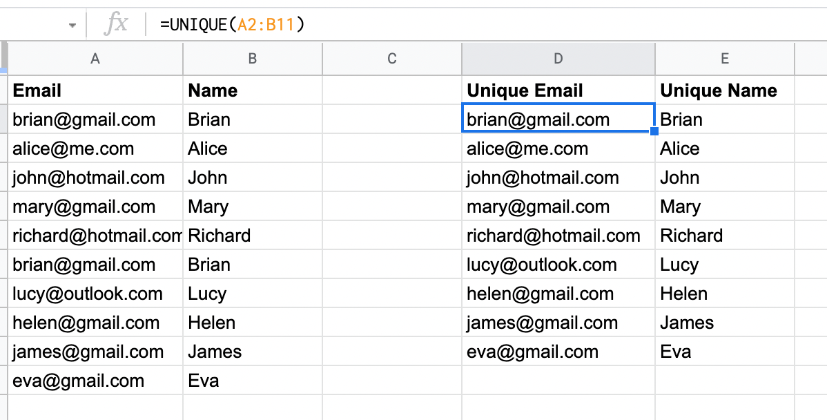
What if you want to also get other columns into your new range? That’s easy to do: simply specify the complete range in the formula above, in my case it will be:

=UNIQUE(A2:B11)

Need help with Google Sheet Formulas? Learn these 9 useful formulas for efficiency.

How to get rid of duplicates in Google Sheets: Summary

Now that we have explained how to filter duplicates in Google Sheets, it is time to summarize all the different methods for easy reference:

1. Use the in-built Remove Duplicates feature of Google Sheets to eliminate duplicates
2. Highlight duplicate values by using conditional formatting
3. Apply the COUNTIF formula to calculate how many times a value is repeated or to indicate the first and repeated instances of the value
4. Try the UNIQUE formula to get unique values into another column(s).